Capstone 2 Evidence Map

Capstone Summary

The provided documentation outlines Capstone 2 of the Microsoft AI Engineering Program 2026, which focuses on data processing and statistical analysis using Python. The project involves importing a previously cleaned healthcare dataset to perform memory usage comparisons and feature scaling, specifically converting encoded age and income variables into real-world units. Students must execute descriptive statistical analysis, identifying significant patterns such as right-skewed distributions in patient visits and financial data. A critical component of the work includes distinguishing between categorical labels and continuous variables to recommend optimal data types for future machine learning tasks. The final requirements necessitate generating a comprehensive report and exporting the modified data as a standardized CSV file for subsequent program modules. These sources collectively serve as a technical evidence map and instructional guide for the capstone's engineering workflow.

Applied Data Science

Capstone 2: Data Processing and Statistical Analysis

Capstone 2 covers memory analysis, scaling, statistical analysis, required CSV export, and reporting.

Mapped source folder: Incremental Capstones/Applied Data Science with Python/Capstone 2

Quick Facts

Input handoff: NSMES1988new.csv
Required output: NSMES1988updated.csv
Memory change from Capstone 1: -35,248 bytes
Scaled analysis fields: age_years, income_dollars

Original Project PDF

The original Capstone 2 directions are embedded here.

Open Viewer Download PDF

Requirement Checklist

The checklist below follows the PDF task sequence.

Import relevant Python libraries.

Source mapping: Notebook C?-T0 and C?-T1

Evidence note: The staged notebook loads runtime path helpers and `pandas` before the Capstone 2 analysis steps begin.

Import the CSV file `NSMES1988new.csv` into a dataframe.

Source mapping: Notebook C?-T2

Evidence note: The notebook loads the Capstone 1 handoff CSV, confirms the path, and previews the dataframe with shape `(4406, 18)`.

Perform memory analysis of the new dataframe and compare it with the memory of the dataframe in the previous week and mark your comments.

Source mapping: Notebook C2-T4

Evidence note: The notebook compares Capstone 2 memory `2,228,671` bytes against the Capstone 1 reference `2,263,919` bytes and records the `-35,248` byte difference.

Perform the following operations on age and income columns: multiply age by 10 and income by 10000.

Source mapping: Notebook C2-T5

Evidence note: The notebook adds `age_years` and `income_dollars` so the scaled values are visible while the original encoded source fields remain available.

Perform basic statistical analysis on the new dataframe and generate a brief report on the outcome.

Source mapping: Notebook C2-T6

Evidence note: The notebook reports descriptive statistics for the numeric fields and summarizes the right-skew behavior of visits and income.

Save the dataframe as `NSMES1988updated.csv` file in the local space for possible future use.

Source mapping: Notebook C2-T7

Evidence note: The required output file is staged at `outputs/NSMES1988updated.csv` with exported shape `(4406, 20)`.

Invoke `describe` command on the dataframe and compare that with the basic statistical analysis done in the previous step.

Source mapping: Notebook C2-T8

Evidence note: The notebook runs `describe(include="all")` and compares that wider summary to the focused statistics from the prior section.

Indicate which of the columns are not eligible for statistical analysis and indicate possible datatype changes, and report.

Source mapping: Notebook C2-T8

Evidence note: The notebook identifies eight label-like fields for categorical treatment and recommends integer downcasts for selected count columns.

Make changes to the recommended file from the previous step and export it as a new `.csv` file for possible future use. Optional.

Source mapping: PDF p.8 optional step

Evidence note: Optional follow-on CSV export is available as `outputs/NSMES1988optimized_optional.csv`.

Prepare a brief report and enter it in the markup cells of the JupyterLab notebook.

Source mapping: Notebook C2-T6, C2-T8, Final section

Evidence note: The notebook markdown cells preserve the brief report and conclusions directly alongside the statistical outputs.

Requirement Walkthrough

Each walkthrough block covers one requirement and the matching notebook evidence.

Runtime and Library Imports

Notebook section: C?-T0 and C?-T1

Requirement: Import relevant Python libraries.

The notebook starts with runtime path handling and imports the dataframe tooling needed for the Capstone 2 analysis path.

Results Capture

Runtime setup establishes reusable project paths and the output folder structure.
`pandas` is imported explicitly for dataframe operations and statistical summaries.
The notebook uses supporting imports in the setup cell instead of scattering them throughout later requirement sections.

from pathlib import Path
from datetime import datetime

try:
    from IPython.display import display
except Exception:
    def display(value):
        print(value)

import pandas as pd

Load the Cleaned Handoff Dataset

Notebook section: C?-T2

Requirement: Import the CSV file `NSMES1988new.csv` into a dataframe.

Capstone 2 begins from the cleaned handoff created at the end of Capstone 1, and the notebook confirms that input path before running any analysis.

Results Capture

Loaded dataset: `NSMES1988new.csv`.
Working dataframe shape: `(4406, 18)`.
A dataframe preview is displayed immediately after load as the first evidence checkpoint.

DEFAULT_DATASET = "NSMES1988new.csv"
DATASET_PATH = resolve_dataset_path(DEFAULT_DATASET)

df = pd.read_csv(DATASET_PATH)
print("Loaded:", DATASET_PATH)
print("Shape:", df.shape)
display(df.head())

Memory Comparison Against Capstone 1

Notebook section: C2-T4

Requirement: Perform memory analysis of the new dataframe and compare it with the memory of the dataframe in the previous week and mark your comments.

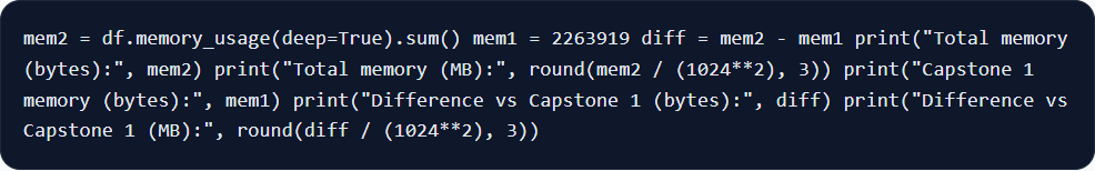
The notebook compares Capstone 2 memory usage to the Capstone 1 reference.

Results Capture

Current dataframe memory: `2,228,671` bytes (`2.125 MB`).
Capstone 1 reference memory: `2,263,919` bytes (`2.159 MB`).
Difference: `-35,248` bytes (`-0.034 MB`), indicating a modest reduction after the cleaned handoff step.

mem2 = df.memory_usage(deep=True).sum()
mem1 = 2263919
diff = mem2 - mem1

print("Total memory (bytes):", mem2)
print("Total memory (MB):", round(mem2 / (1024**2), 3))
print("Capstone 1 memory (bytes):", mem1)
print("Difference vs Capstone 1 (bytes):", diff)
print("Difference vs Capstone 1 (MB):", round(diff / (1024**2), 3))

Scale Age and Income to Real Units

Notebook section: C2-T5

Requirement: Perform the following operations on age and income columns: multiply age by 10 and income by 10000.

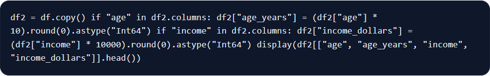
The notebook adds scaled columns while keeping the original encoded source fields.

Results Capture

`age` stays available as the original encoded field while `age_years` exposes the real-year values.
`income` stays available as the original encoded field while `income_dollars` exposes dollar values.
Scaled ranges: `age_years` from `66` to `109`; `income_dollars` from `-10,125` to `548,351`.

df2 = df.copy()

if "age" in df2.columns:
    df2["age_years"] = (df2["age"] * 10).round(0).astype("Int64")

if "income" in df2.columns:
    df2["income_dollars"] = (df2["income"] * 10000).round(0).astype("Int64")

display(df2[["age", "age_years", "income", "income_dollars"]].head())

Basic Statistical Analysis and Brief Report

Notebook section: C2-T6

Requirement: Perform basic statistical analysis on the new dataframe and generate a brief report on the outcome.

The notebook combines numeric summary tables with a written interpretation of the distribution patterns that matter most for the dataset.

Results Capture

`visits` summary: mean `5.774`, median `4`, min `0`, max `89`.
`age_years` summary: mean `74.024`, median `73`, min `66`, max `109`.
`income_dollars` summary: mean `25,271.321`, median `16,981.5`, min `-10,125`, max `548,351`.
The notebook report notes right-skew in utilization and income, and it retains the negative-income records.

numeric_cols = df2.select_dtypes(include=["number"]).columns
display(df2[numeric_cols].describe())

summary = df2[["visits", "age_years", "income_dollars"]].agg(["mean", "median", "min", "max"]).T
display(summary)

Export the Updated Handoff File

Notebook section: C2-T7

Requirement: Save the dataframe as `NSMES1988updated.csv` file in the local space for possible future use.

After the scaling step and statistical summary work are complete, the notebook exports the updated dataset for downstream capstone use.

Results Capture

Saved file: `outputs/NSMES1988updated.csv`.
Exported dataframe shape: `(4406, 20)`.
The exported file carries the original 18 fields plus `age_years` and `income_dollars`.

out_csv = OUTPUT_DIR / "NSMES1988updated.csv"
df2.to_csv(out_csv, index=False)
print("Saved:", out_csv)
print("Shape:", df2.shape)

Compare `describe()` With the Prior Summary

Notebook section: C2-T8

Requirement: Invoke `describe` command on the dataframe and compare that with the basic statistical analysis done in the previous step.

The notebook widens the statistical view by running `describe(include="all")`, then compares that broader output to the focused summaries already written for visits, age, and income.

Results Capture

The broader `describe()` output confirms the same central tendencies surfaced in the focused summary section.
The all-column view adds category counts and top values for label-like fields that were not part of the narrower numeric-only report.
This step compares the `describe()` output with the earlier brief report.

display(df2.describe(include="all"))

summary = df2[["visits", "age_years", "income_dollars"]].agg(["mean", "median", "min", "max"]).T
display(summary)

Identify Non-Eligible Fields and Dtype Changes

Notebook section: C2-T8

Requirement: Indicate which of the columns are not eligible for statistical analysis and indicate possible datatype changes, and report.

The notebook separates fields that are label-like from fields that are suitable for continuous analysis and records concrete dtype recommendations for each group.

Results Capture

Columns not eligible for continuous numeric interpretation: `health`, `adl`, `region`, `gender`, `married`, `employed`, `insurance`, `medicaid`.
Recommended `category` conversions match those eight label and flag fields.
Recommended downcasts: `int8` for `visits`, `nvisits`, `emergency`, `hospital`, `chronic`, `school`, `age_years`; `int16` for `ovisits` and `novisits`.

cat_like = ["health", "adl", "region", "gender", "married", "employed", "insurance", "medicaid"]
print("Categorical/label-like columns:", cat_like)

recommend_rows = []
for column_name in cat_like:
    recommend_rows.append({
        "column": column_name,
        "eligible_for_continuous_stats": "No",
        "suggested_dtype": "category",
    })

display(pd.DataFrame(recommend_rows))

Optional Follow-On CSV Export

Notebook section: PDF p.8 optional step

Requirement: Make changes to the recommended file from the previous step and export it as a new `.csv` file for possible future use. Optional.

An optional follow-on CSV export is available.

Results Capture

Optional artifact: `outputs/NSMES1988optimized_optional.csv`.
This optional export is tracked separately from the required `NSMES1988updated.csv` handoff file.
This export is optional.

# Optional follow-on export
optional_out_csv = OUTPUT_DIR / "NSMES1988optimized_optional.csv"
print("Saved:", optional_out_csv)

Notebook Report in Markup Cells

Notebook section: C2-T6, C2-T8, Final section

Requirement: Prepare a brief report and enter it in the markup cells of the JupyterLab notebook.

Capstone 2 closes with notebook markdown blocks that interpret the statistical outputs and restate the capstone outcome in narrative form.

Results Capture

The notebook records a brief report after the basic statistical analysis section.
The notebook restates the field eligibility and dtype recommendations in markdown alongside the tables.
The final markdown section summarizes the memory comparison, the new scaled fields, and the updated CSV output artifact.

Visit counts are right-skewed, with a small high-utilization tail.
The sample is concentrated in older age bands, with a median age of 73 years.
Income is highly right-skewed, so the median is more robust than the mean.
Negative income values are preserved and documented instead of being dropped blindly.

Open the optional follow-on CSV export derived from the dtype recommendation step.

View Download

Colab Notebook

This section provides the notebook preview, launch link, and project file links.

Capstone 2 input and output files remain available on this page.

Embedded Notebook Preview

Cell 1 Markdown

Capstone 2 — Session 2: Data Processing and Statistical Analysis

Run timestamp: 2026-02-19 01:49:22

Goal

Process the cleaned NSMES dataset from Capstone 1, transform encoded variables (age, income) into real-world units, and produce a statistically summarized dataset for downstream modeling.
Deliver documented evidence for memory comparison, transformation correctness, descriptive statistics, and export readiness for Capstone 3.

Inputs

NSMES1988new.csv (copied from Capstone 1 outputs if not already present locally)

Outputs

All exports go to ./outputs/ (and plots to ./outputs/plots/ when applicable)

Libraries (documented)

pandas: needed for DataFrame operations and descriptive statistics; enabled loading, transforming, validating, and exporting tabular data.

Key dataset note

age is encoded as Age in years (divided by 10) (e.g., 6.9 = 69 years).

Cell 2 Markdown

C?-T0 - Runtime setup (local + Colab paths)

This setup cell prepares reproducible working folders for local runs and Google Colab.

When the notebook runs in Colab, it stages the PDF, notebook copy, and input CSV files from the public Francis Burnet GitHub repository before the requirement steps begin.

Cell 3 Code · python

from pathlib import Path
from datetime import datetime
from urllib.parse import quote
from urllib.request import urlretrieve
import os
import sys

try:
    from IPython.display import display
except Exception:
    def display(value):
        print(value)

# --- Project metadata ---
CAPSTONE = 2
SESSION_TITLE = 'Session 2: Data Processing and Statistical Analysis'
IS_COLAB = 'google.colab' in sys.modules
RAW_BASE = os.environ.get('FRANCISBURNET_RAW_BASE', 'https://raw.githubusercontent.com/FrancisBurnet/francisburnet/main')

print(f"Capstone: {CAPSTONE} | Session: {SESSION_TITLE}")
print("Run timestamp:", datetime.now().strftime("%Y-%m-%d %H:%M:%S"))
print("Runtime:", "Google Colab" if IS_COLAB else "Local / notebook runtime")

CWD = Path.cwd()
if IS_COLAB:
    BASE_DIR = Path('/content/francisburnet_capstone_2')
elif (CWD / f"Capstone {CAPSTONE}").exists():
    BASE_DIR = CWD / f"Capstone {CAPSTONE}"
elif CWD.name == f"Capstone {CAPSTONE}":
    BASE_DIR = CWD
elif (CWD / 'Incremental_Capstone' / f"Capstone {CAPSTONE}").exists():
    BASE_DIR = CWD / 'Incremental_Capstone' / f"Capstone {CAPSTONE}"
else:
    BASE_DIR = CWD

INPUT_DIR = BASE_DIR / 'inputs'
OUTPUT_DIR = BASE_DIR / 'outputs'
PLOTS_DIR = OUTPUT_DIR / 'plots'
INPUT_DIR.mkdir(parents=True, exist_ok=True)
OUTPUT_DIR.mkdir(parents=True, exist_ok=True)
PLOTS_DIR.mkdir(parents=True, exist_ok=True)

# --- Paths ---
def first_existing_path(candidates):
    for candidate in candidates:
        candidate = Path(candidate).expanduser()
        if candidate.exists():
            return candidate
    return None

def github_raw_url(relative_path: str) -> str:
    normalized = relative_path.replace('\\', '/')
    return RAW_BASE.rstrip('/') + '/' + quote(normalized, safe='/')

def stage_colab_asset(relative_path: str, destination_name=None) -> Path:
    destination = INPUT_DIR / (destination_name or Path(relative_path).name)
    if not destination.exists():
        asset_url = github_raw_url(relative_path)
        urlretrieve(asset_url, destination)
        print('Downloaded:', destination.name, 'from', asset_url)
    return destination

def resolve_dataset_path(default_filename: str) -> Path:
    """Resolve dataset path from local folders or the Colab staging folder."""
    path = first_existing_path([
        INPUT_DIR / default_filename,
        BASE_DIR / default_filename,
        CWD / default_filename,
        CWD / 'Incremental_Capstone' / f"Capstone {CAPSTONE}" / default_filename,
    ])
    if path is None:
        searched_paths = [
            str(INPUT_DIR / default_filename),
            str(BASE_DIR / default_filename),
            str(CWD / default_filename),
            str(CWD / 'Incremental_Capstone' / f"Capstone {CAPSTONE}" / default_filename),
        ]
        raise FileNotFoundError(
            f"Dataset not found: {default_filename}. Searched: {searched_paths}"
        )
    return path

if IS_COLAB:
    staged_assets = [
        'Incremental Capstones/Applied Data Science with Python/Capstone 2/Capstone_Session_2.pdf',
        'Incremental Capstones/Applied Data Science with Python/Capstone 2/NSMES1988.csv',
        'Incremental Capstones/Applied Data Science with Python/Capstone 2/NSMES1988new.csv',
        'Incremental Capstones/Applied Data Science with Python/Capstone 2/capstone_2.ipynb',
    ]
    for relative_path in staged_assets:
        stage_colab_asset(relative_path)

print('Base directory:', BASE_DIR)
print('Input directory:', INPUT_DIR)
print('Output directory:', OUTPUT_DIR)
print('Plots directory:', PLOTS_DIR)

Output

Capstone: 2 | Session: Session 2: Data Processing and Statistical Analysis
Run timestamp: 2026-02-19 00:31:20
Output directory: c:\DEV_Projects\SIMPLILEARN\CAPSTONE_Applied_Data_Science_with _Python\Incremental_Capstone\Capstone 2\outputs
Plots directory: c:\DEV_Projects\SIMPLILEARN\CAPSTONE_Applied_Data_Science_with _Python\Incremental_Capstone\Capstone 2\outputs\plots

Cell 4 Markdown

C?-T1 — Imports (ONLY what you use)

I documented each import with why I used it and what it enabled in this capstone.

Cell 5 Code · python

import pandas as pd  # DataFrames + CSV/JSON IO + analysis tables

Cell 6 Markdown

C?-T2 - Load dataset

This step loads the required Capstone 2 input file from the local project folder or the Colab staging folder created in setup.

Cell 7 Code · python

DEFAULT_DATASET = 'NSMES1988new.csv'

try:
    dataset_path = resolve_dataset_path(DEFAULT_DATASET)
except FileNotFoundError:
    fallback = first_existing_path([
        BASE_DIR.parent / 'Capstone 1' / 'outputs' / 'NSMES1988new.csv',
        CWD / 'Capstone 1' / 'outputs' / 'NSMES1988new.csv',
        CWD / 'Incremental_Capstone' / 'Capstone 1' / 'outputs' / 'NSMES1988new.csv',
    ])
    if fallback is None and IS_COLAB:
        fallback = stage_colab_asset(
            'Incremental Capstones/Applied Data Science with Python/Capstone 2/NSMES1988new.csv'
        )
    if fallback is None:
        raise
    dataset_path = fallback
    print('Default dataset not found; using fallback:', dataset_path)

df = pd.read_csv(dataset_path)

print('Loaded:', dataset_path)
print('Shape:', df.shape)
display(df.head())

Output

Loaded: c:\DEV_Projects\SIMPLILEARN\CAPSTONE_Applied_Data_Science_with _Python\Incremental_Capstone\Capstone 2\NSMES1988new.csv
Shape: (4406, 18)

   visits  nvisits  ovisits  novisits  emergency  hospital   health  chronic  \
0       5        0        0         0          0         1  average        2   
1       1        0        2         0          2         0  average        2   
2      13        0        0         0          3         3     poor        4   
3      16        0        5         0          1         1     poor        2   
4       3        0        0         0          0         0  average        2   

       adl region  age  gender married  school  income employed insurance  \
0   normal  other  6.9    male     yes       6  2.8810      yes       yes   
1   normal  other  7.4  female     yes      10  2.7478       no       yes   
2  limited  other  6.6  female      no      10  0.6532       no        no   
3  limited  other  7.6    male     yes       3  0.6588       no       yes   
4  limited  other  7.9  female     yes       6  0.6588       no       yes   

  medicaid  
0       no  
1       no  
2      yes  
3       no  
4       no

Cell 8 Markdown

C?-T3 — Validation checks

Confirm expected columns exist
Confirm key dtypes
Check missing values

Results Capture:

What I did: I validated expected schema, reviewed dtypes, and computed missing-value counts across all columns.
What I found: all expected 18 columns are present, no missing values were detected, and age/income are numeric (float64) as required for scaling.
Caveats: categorical concepts (e.g., region, gender) are integer-encoded and should be interpreted as labels, not continuous measures.

Cell 9 Code · python

expected_cols = [
    "visits", "nvisits", "ovisits", "novisits", "emergency", "hospital",
    "health", "chronic", "adl", "region", "age", "gender",
    "married", "school", "income", "employed", "insurance", "medicaid"
]

missing_cols = [c for c in expected_cols if c not in df.columns]
print("Missing expected columns:", missing_cols)

print("\nDtypes:")
display(df.dtypes)

print("\nMissing values (count):")
na_counts = df.isna().sum().sort_values(ascending=False)
display(na_counts[na_counts > 0] if (na_counts > 0).any() else na_counts.head())

Output

Missing expected columns: []

Dtypes:

visits         int64
nvisits        int64
ovisits        int64
novisits       int64
emergency      int64
hospital       int64
health           str
chronic        int64
adl              str
region           str
age          float64
gender           str
married          str
school         int64
income       float64
employed         str
insurance        str
medicaid         str
dtype: object

Missing values (count):

visits       0
nvisits      0
ovisits      0
novisits     0
emergency    0
dtype: int64

Cell 10 Markdown

C2-T4 — Load NSMES1988new.csv and compare memory with Week 1

PDF requirement: Import NSMES1988new.csv and provide memory analysis compared to Week 1.

What I completed

I loaded NSMES1988new.csv, measured memory usage, and compared it against Capstone 1 memory evidence.

Results Capture

Current dataframe memory: 2,228,671 bytes (2.125 MB).
Capstone 1 memory reference: 2,263,919 bytes (2.159 MB).
Difference: -35,248 bytes (-0.034 MB), indicating a modest reduction from Week 1 after the cleaned-schema handoff.

Code evidence

The next cell shows the exact memory comparison code I executed.

Cell 11 Code · python

# Memory comparison against Capstone 1 reference

mem2 = df.memory_usage(deep=True).sum()
mem1 = 2263919  # from Capstone 1 WORK_SUMMARY
diff = mem2 - mem1
print("Total memory (bytes):", mem2)
print("Total memory (MB):", round(mem2 / (1024**2), 3))
print("Capstone 1 memory (bytes):", mem1)
print("Difference vs Capstone 1 (bytes):", diff)
print("Difference vs Capstone 1 (MB):", round(diff / (1024**2), 3))

Output

Total memory (bytes): 2228671
Total memory (MB): 2.125
Capstone 1 memory (bytes): 2263919
Difference vs Capstone 1 (bytes): -35248
Difference vs Capstone 1 (MB): -0.034

Cell 12 Markdown

C2-T5 — Transform age and income (scale to real units)

PDF requirement: Multiply age by 10 and income by 10000.

What I completed

I created age_years and income_dollars to preserve raw values while adding real-unit scaled fields.

Results Capture

age before scaling: min=6.6, max=10.9 → age_years after scaling: min=66, max=109.

income before scaling: min=-1.0125, max=54.8351 → income_dollars after scaling: min=-10,125, max=548,351.

New columns preserve raw source fields while exposing interpretable units for analysis.

Code evidence

The next cell contains the exact transformation logic and preview output.

Cell 13 Code · python

# Transformations (recommended: keep raw + create scaled)
df2 = df.copy()

if "age" in df2.columns:
    df2["age_years"] = (df2["age"] * 10).round(0).astype("Int64")

if "income" in df2.columns:
    df2["income_dollars"] = (df2["income"] * 10000).round(0).astype("Int64")

cols = [c for c in ["age","age_years","income","income_dollars"] if c in df2.columns]
display(df2[cols].head())

Output

   age  age_years  income  income_dollars
0  6.9         69  2.8810           28810
1  7.4         74  2.7478           27478
2  6.6         66  0.6532            6532
3  7.6         76  0.6588            6588
4  7.9         79  0.6588            6588

Cell 14 Markdown

C2-T6 — Basic statistical analysis + brief report

PDF requirement: Provide basic statistical analysis and a brief report on the dataset.

What I completed

I computed descriptive statistics and interpreted the key metrics for visits, age, and income.

Results Capture

Key stats (mean | median | min | max):

visits: 5.774 | 4.0 | 0 | 89

age_years: 74.024 | 73.0 | 66 | 109

income_dollars: 25,271.321 | 16,981.5 | -10,125 | 548,351

Brief report:

Visit counts are right-skewed (mean > median), with a small high-utilization tail.

The sample is concentrated in older age bands (median 73 years).

Income is highly right-skewed with a large upper tail, so median is more robust than mean.

Negative income values appear and should be preserved/documented rather than dropped blindly.

Scaled features (age_years, income_dollars) are now directly interpretable in business terms.

Code evidence

The next cell contains the descriptive summary tables used in this report.

Cell 15 Code · python

# Basic stats
numeric_cols = df2.select_dtypes(include=["number"]).columns
display(df2[numeric_cols].describe())

summary = df2[["visits", "age_years", "income_dollars"]].agg(["mean", "median", "min", "max"]).T
display(summary)

Output

            visits      nvisits      ovisits     novisits    emergency  \
count  4406.000000  4406.000000  4406.000000  4406.000000  4406.000000   
mean      5.774399     1.618021     0.750794     0.536087     0.263504   
std       6.759225     5.317056     3.652759     3.879506     0.703659   
min       0.000000     0.000000     0.000000     0.000000     0.000000   
25%       1.000000     0.000000     0.000000     0.000000     0.000000   
50%       4.000000     0.000000     0.000000     0.000000     0.000000   
75%       8.000000     1.000000     0.000000     0.000000     0.000000   
max      89.000000   104.000000   141.000000   155.000000    12.000000   

          hospital      chronic          age       school       income  \
count  4406.000000  4406.000000  4406.000000  4406.000000  4406.000000   
mean      0.295960     1.541988     7.402406    10.290286     2.527132   
std       0.746398     1.349632     0.633405     3.738736     2.924648   
min       0.000000     0.000000     6.600000     0.000000    -1.012500   
25%       0.000000     1.000000     6.900000     8.000000     0.912150   
50%       0.000000     1.000000     7.300000    11.000000     1.698150   
75%       0.000000     2.000000     7.800000    12.000000     3.172850   
max       8.000000     8.000000    10.900000    18.000000    54.835100   

       age_years  income_dollars  
count     4406.0          4406.0  
mean   74.024058    25271.320699  
std      6.33405    29246.475762  
min         66.0        -10125.0  
25%         69.0          9121.5  
50%         73.0         16981.5  
75%         78.0         31728.5  
max        109.0        548351.0

                        mean   median      min       max
visits              5.774399      4.0      0.0      89.0
age_years          74.024058     73.0     66.0     109.0
income_dollars  25271.320699  16981.5 -10125.0  548351.0

Cell 16 Markdown

C2-T7 — Export updated dataset for next capstone

PDF requirement: Export as NSMES1988updated.csv.

What I completed

I exported the transformed dataframe to the required handoff file for Capstone 3.

Results Capture

Saved file: outputs/NSMES1988updated.csv.
Exported shape: (4406, 20) with two added columns (age_years, income_dollars).

Artifacts

outputs/NSMES1988updated.csv

Code evidence

The next cell contains the export command and shape confirmation output.

Cell 17 Code · python

out_csv = OUTPUT_DIR / "NSMES1988updated.csv"
df2.to_csv(out_csv, index=False)
print("Saved:", out_csv)
print("Shape:", df2.shape)

Output

Saved: c:\DEV_Projects\SIMPLILEARN\CAPSTONE_Applied_Data_Science_with _Python\Incremental_Capstone\Capstone 2\outputs\NSMES1988updated.csv
Shape: (4406, 20)

Cell 18 Markdown

C2-T8 — Describe() comparison + identify non-eligible columns

PDF requirement: Use describe() and compare; identify columns not eligible for statistical analysis and recommend dtype changes.

What I completed

I ran numeric/all-column describe comparisons and documented non-eligible columns plus dtype recommendations.

Results Capture

Non-eligible for continuous numeric interpretation: health, adl, region, gender, married, employed, insurance, medicaid (encoded labels/flags where mean/std are not substantively meaningful).
Dtype recommendations:
category: health, adl, region, gender, married, employed, insurance, medicaid
Small integer optimization candidates: visits, nvisits, emergency, hospital, chronic, school, age_years → int8; ovisits, novisits → int16 (after validation in production pipeline).

Code evidence

The next cell shows the full comparison output and recommendation table.

Cell 19 Code · python

# Describe comparison
display(df2.describe(include="all"))

cat_like = ["health", "adl", "region", "gender", "married", "employed", "insurance", "medicaid"]
print("Categorical/label-like columns:", cat_like)

recommend_rows = []
for c in cat_like:
    recommend_rows.append({
        "column": c,
        "eligible_for_continuous_stats": "No",
        "suggested_dtype": "category",
        "reason": "Encoded category/flag; arithmetic moments are weakly interpretable"
    })

for c in ["visits", "nvisits", "emergency", "hospital", "chronic", "school", "age_years"]:
    recommend_rows.append({
        "column": c,
        "eligible_for_continuous_stats": "Yes",
        "suggested_dtype": "int8",
        "reason": "Observed range fits int8; optimize memory"
    })

for c in ["ovisits", "novisits"]:
    recommend_rows.append({
        "column": c,
        "eligible_for_continuous_stats": "Yes",
        "suggested_dtype": "int16",
        "reason": "Observed range fits int16"
    })

display(pd.DataFrame(recommend_rows))

Output

             visits      nvisits      ovisits     novisits    emergency  \
count   4406.000000  4406.000000  4406.000000  4406.000000  4406.000000   
unique          NaN          NaN          NaN          NaN          NaN   
top             NaN          NaN          NaN          NaN          NaN   
freq            NaN          NaN          NaN          NaN          NaN   
mean       5.774399     1.618021     0.750794     0.536087     0.263504   
std        6.759225     5.317056     3.652759     3.879506     0.703659   
min        0.000000     0.000000     0.000000     0.000000     0.000000   
25%        1.000000     0.000000     0.000000     0.000000     0.000000   
50%        4.000000     0.000000     0.000000     0.000000     0.000000   
75%        8.000000     1.000000     0.000000     0.000000     0.000000   
max       89.000000   104.000000   141.000000   155.000000    12.000000   

           hospital   health      chronic     adl region          age  gender  \
count   4406.000000     4406  4406.000000    4406   4406  4406.000000    4406   
unique          NaN        3          NaN       2      4          NaN       2   
top             NaN  average          NaN  normal  other          NaN  female   
freq            NaN     3509          NaN    3507   1614          NaN    2628   
mean       0.295960      NaN     1.541988     NaN    NaN     7.402406     NaN   
std        0.746398      NaN     1.349632     NaN    NaN     0.633405     NaN   
min        0.000000      NaN     0.000000     NaN    NaN     6.600000     NaN   
25%        0.000000      NaN     1.000000     NaN    NaN     6.900000     NaN   
50%        0.000000      NaN     1.000000     NaN    NaN     7.300000     NaN   
75%        0.000000      NaN     2.000000     NaN    NaN     7.800000     NaN   
max        8.000000      NaN     8.000000     NaN    NaN    10.900000     NaN   

       married       school       income employed insurance medicaid  \
count     4406  4406.000000  4406.000000     4406      4406     4406   
unique       2          NaN          NaN        2         2        2   
top        yes          NaN          NaN       no       yes       no   
freq      2406          NaN          NaN     3951      3421     4004   
mean       NaN    10.290286     2.527132      NaN       NaN      NaN   
std        NaN     3.738736     2.924648      NaN       NaN      NaN   
min        NaN     0.000000    -1.012500      NaN       NaN      NaN   
25%        NaN     8.000000     0.912150      NaN       NaN      NaN   
50%        NaN    11.000000     1.698150      NaN       NaN      NaN   
75%        NaN    12.000000     3.172850      NaN       NaN      NaN   
max        NaN    18.000000    54.835100      NaN       NaN      NaN   

        age_years  income_dollars  
count      4406.0          4406.0  
unique       <NA>            <NA>  
top          <NA>            <NA>  
freq         <NA>            <NA>  
mean    74.024058    25271.320699  
std       6.33405    29246.475762  
min          66.0        -10125.0  
25%          69.0          9121.5  
50%          73.0         16981.5  
75%          78.0         31728.5  
max         109.0        548351.0

Categorical/label-like columns: ['health', 'adl', 'region', 'gender', 'married', 'employed', 'insurance', 'medicaid']

       column eligible_for_continuous_stats suggested_dtype  \
0      health                            No        category   
1         adl                            No        category   
2      region                            No        category   
3      gender                            No        category   
4     married                            No        category   
5    employed                            No        category   
6   insurance                            No        category   
7    medicaid                            No        category   
8      visits                           Yes            int8   
9     nvisits                           Yes            int8   
10  emergency                           Yes            int8   
11   hospital                           Yes            int8   
12    chronic                           Yes            int8   
13     school                           Yes            int8   
14  age_years                           Yes            int8   
15    ovisits                           Yes           int16   
16   novisits                           Yes           int16   

                                               reason  
0   Encoded category/flag; arithmetic moments are ...  
1   Encoded category/flag; arithmetic moments are ...  
2   Encoded category/flag; arithmetic moments are ...  
3   Encoded category/flag; arithmetic moments are ...  
4   Encoded category/flag; arithmetic moments are ...  
5   Encoded category/flag; arithmetic moments are ...  
6   Encoded category/flag; arithmetic moments are ...  
7   Encoded category/flag; arithmetic moments are ...  
8           Observed range fits int8; optimize memory  
9           Observed range fits int8; optimize memory  
10          Observed range fits int8; optimize memory  
11          Observed range fits int8; optimize memory  
12          Observed range fits int8; optimize memory  
13          Observed range fits int8; optimize memory  
14          Observed range fits int8; optimize memory  
15                          Observed range fits int16  
16                          Observed range fits int16

Cell 20 Markdown

Final section — Conclusions (required)

I successfully processed the Capstone 1 cleaned dataset and prepared it for downstream use.
I observed a slightly lower memory footprint than Week 1 (2.125 MB vs 2.159 MB).
I made age and income directly interpretable by adding age_years and income_dollars.
I documented right-skew patterns in utilization and income distributions.
I identified categorical/flag columns suitable for category typing and non-continuous interpretation.
I produced the required artifact: outputs/NSMES1988updated.csv.
I updated WORK_SUMMARY.md with evidence and marked all Capstone 2 tasks complete.

Cell 21 Code · python

print("Capstone 2 completed: C2-T4 to C2-T8")
print("Primary artifact: outputs/NSMES1988updated.csv")

Output

Capstone 2 completed: C2-T4 to C2-T8
Primary artifact: outputs/NSMES1988updated.csv

Project Notes

Notebook preview and launch link.
Input handoff dataset and required output CSV.
Optional follow-on CSV when available.
Capstone 2 notebook workspace.

Launch Controls

Notebook Launch

Launch the matching notebook in Google Colab or open the source file.

Launch Colab View Notebook Source

Project File Links

Input Handoff Dataset: Open Input Handoff Dataset
The cleaned Capstone 1 handoff file that Capstone 2 loads as its working input.
Notebook File: Open Notebook File
The staged Capstone 2 notebook used as the main evidence source for the walkthrough.
Updated Output CSV: Open Updated Output CSV
The required Capstone 2 output file produced after the scaling and statistical analysis steps.
Optional Follow-On CSV: Open Optional Follow-On CSV
Optional follow-on export derived from the dtype recommendation step.
Notebook Source: Open Notebook Source
Public GitHub source path used for the site-backed Colab launch flow.
Project Infographic: Open Project Infographic
Portfolio-ready visual summary for the Capstone 2 workflow and staged deliverables.

Colab and source links follow the configured notebook path.

Execution Notes

Current mode: notebook-backed presentation with downloadable artifacts.

This page presents the PDF, notebook, input dataset, and exported outputs.

The notebook opens in Google Colab when launched.