Capstone Project
Capstone 7
Machine learning capstone page covering unsupervised analysis, visuals, and saved outputs.
Capstone 7 Scope
Capstone 7 turns the copied clustering assignment into an executed PCA and KMeans workflow with saved variance, elbow, and cluster-scatter outputs.
Primary staged dataset: CC GENERAL.csv.
Notebook evidence plus covariance, cluster assignment, and summary exports are staged under outputs/.
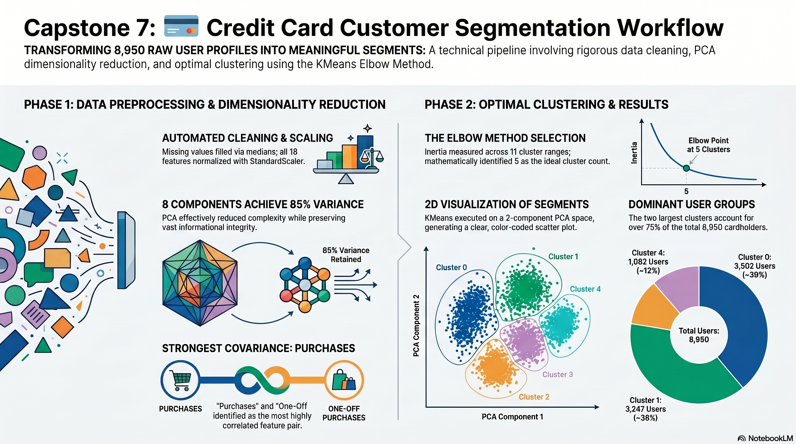
Capstone 7 Infographic
This visual summary sits alongside the detailed walkthrough so the project can be understood quickly before drilling into the notebook, metrics, and exported artifacts.
Original Project PDF
The copied project directions are embedded here for direct comparison against the notebook and output artifacts.
Requirement Checklist
1a
Cluster the credit card users into different groups to find meaningful patterns.
Source mapping: Requirements file
1b
Use Principal Component Analysis (PCA) to reduce the dimension of the feature space.
Source mapping: Requirements file
1j
Plot number of components versus PCA cumulative explained variance.
Source mapping: Requirements file
1k
Identify the number of components required to cover 85 percent of the variance.
Source mapping: Requirements file
1l
Perform PCA with 2 principal components for clustering visualization.
Source mapping: Requirements file
1m
Find the 2 columns that give the most covariances.
Source mapping: Requirements file
1n
Interpret the PCA results by looking at the covariance matrix using `get_covariance()`.
Source mapping: Requirements file
1o
Perform K Means clustering on the 2-component PCA transformed data with clusters ranging from 2 to 11.
Source mapping: Requirements file
1p
Plot K Means inertia against the number of clusters using the Elbow Method.
Source mapping: Requirements file
1q
Identify the ideal number of clusters from the elbow plot.
Source mapping: Requirements file
1r
Perform K Means clustering on the 2-component PCA transformed data using the ideal number of clusters.
Source mapping: Requirements file
1s
Visualize the clusters on a scatter plot between the 1st and 2nd PCA components using different colors for each cluster.
Source mapping: Requirements file
Requirement Walkthrough
Each walkthrough block maps the copied PDF requirements to the executed notebook cells, exported outputs, and reviewable evidence staged with this capstone.
7a
Clean The Credit Card Dataset And Scale The Features
Notebook section: Load, null-handling, and scaling cells
Requirement: Load the dataset, check nulls, handle missing values, and apply StandardScaler before PCA.
The notebook removes the identifier column, fills the missing credit-limit and minimum-payment fields with medians, and scales the remaining numeric feature set for PCA.
Results Capture
- Missing-value counts filled: {"MINIMUM_PAYMENTS":313,"CREDIT_LIMIT":1}.
- Scaling is applied to the full feature matrix before PCA fitting.
working_df = df.drop(columns=['CUST_ID']).copy()
for column in working_df.columns:
    if working_df[column].isna().any():
        working_df[column] = working_df[column].fillna(working_df[column].median())
scaled = scaler.fit_transform(working_df)
7b
Use PCA To Measure Variance Coverage And Covariance
Notebook section: Full PCA and covariance cells
Requirement: Plot cumulative explained variance, identify the components covering 85% of variance, and inspect covariance structure.
The notebook exports the cumulative explained-variance curve, records the component count needed to cover 85% variance, and saves the PCA covariance matrix as a CSV artifact.
Results Capture
- Components needed to cover 85% variance: 8.
- Top covariance pair: PURCHASES and ONEOFF_PURCHASES.
pca_full = PCA()
pca_full.fit(scaled)
explained = np.cumsum(pca_full.explained_variance_ratio_)
components_needed = int(np.argmax(explained >= 0.85) + 1)
Associated Artifact
PCA Explained Variance
Saved cumulative explained-variance chart.

Associated Artifact
KMeans Elbow
Saved elbow-method chart for cluster count selection.

7c
Run KMeans And Visualize The Final Clusters
Notebook section: KMeans clustering and scatter-plot cells
Requirement: Use the elbow method to select the cluster count, run KMeans on the 2-component PCA space, and plot the clusters.
The notebook measures inertia across 2 to 11 clusters, selects the elbow point, and exports the final 2D PCA scatter plot plus the cluster assignments CSV.
Results Capture
- Selected cluster count: 5.
- Cluster-size summary: [3502,3247,1038,81,1082].
- Cluster assignments are exported as CSV for site review.
final_model = KMeans(n_clusters=ideal_clusters, random_state=42, n_init=20)
clusters = final_model.fit_predict(pca_features)
cluster_df = pd.DataFrame({'pca_1': pca_features[:, 0], 'pca_2': pca_features[:, 1], 'cluster': clusters})
Associated Artifact
Cluster Scatter Plot
Saved 2D PCA cluster scatter plot.

Data And Artifact Links
The links below open the copied project files, executed notebook, generated outputs, and staged evidence artifacts for this capstone.
Artifact
Project PDF
Open the copied project directions PDF for this capstone.
Artifact
Notebook Evidence
View the notebook as a readable page or download the original file.
Artifact
Requirements File
Open the generated requirements file for the website workflow.
Artifact
Original CSV Dataset
View the original source CSV staged for this capstone or download the raw file.
Artifact
Project Infographic
Open the infographic summary that visually explains this capstone.
Artifact
JSON Output
Open the generated JSON artifact or download the original file.
Artifact
CSV Output
Open the generated CSV handoff or download the original file.
Artifact
Cluster Assignments CSV
Exported cluster labels in PCA space.
Artifact
Covariance Matrix CSV
Exported PCA covariance matrix for the feature set.
Artifact
Summary JSON
Structured summary of PCA coverage, top covariance pair, and cluster sizes.
Colab Notebook
This section provides the notebook preview, launch link, and project file links.
The notebook opens in Google Colab when a launch URL is configured, and the project files and outputs remain available here on the site.
Embedded Notebook Preview
Cell 1 Markdown
Capstone Session 7
This notebook is generated from the copied Capstone_Session_7.pdf directions and the staged CC GENERAL.csv dataset.
Cell 2 Markdown
Objective
Cluster credit card users using PCA and K-means while preserving the requirement order from the copied PDF.
Cell 3 Code · python
from pathlib import Path
import json
import sys
from urllib.parse import quote

import matplotlib.pyplot as plt
import numpy as np
import pandas as pd
import seaborn as sns
from IPython.display import display
from sklearn.cluster import KMeans
from sklearn.decomposition import PCA
from sklearn.preprocessing import StandardScaler

IS_COLAB = 'google.colab' in sys.modules
GITHUB_REPO_OWNER = 'FrancisBurnet'
GITHUB_REPO_NAME = 'francisburnet'
GITHUB_REPO_BRANCH = 'main'
CAPSTONE_ROOT = Path('Incremental Capstones/Machine Learning Using Python/Capstone Session 7')
DATASET_FILENAME = 'CC GENERAL.csv'


def build_raw_github_url(relative_path: Path) -> str:
    encoded_path = quote(relative_path.as_posix(), safe='/')
    return (
        f"https://raw.githubusercontent.com/{GITHUB_REPO_OWNER}/{GITHUB_REPO_NAME}/"
        f"{GITHUB_REPO_BRANCH}/{encoded_path}"
    )


def resolve_capstone_dir() -> Path | None:
    current = Path.cwd().resolve()
    capstone_parts = CAPSTONE_ROOT.parts
    for candidate in [current, *current.parents]:
        if len(candidate.parts) >= len(capstone_parts) and candidate.parts[-len(capstone_parts):] == capstone_parts:
            return candidate
        nested_candidate = candidate / CAPSTONE_ROOT
        if nested_candidate.exists():
            return nested_candidate
    return None


CAPSTONE_DIR = resolve_capstone_dir()
DATASET_URL = build_raw_github_url(CAPSTONE_ROOT / DATASET_FILENAME)

if CAPSTONE_DIR is not None:
    OUTPUT_ROOT = CAPSTONE_DIR
    OUTPUT_MODE = 'permanent capstone outputs'
    OUTPUT_DISPLAY = (CAPSTONE_ROOT / 'outputs').as_posix()
else:
    runtime_root = Path('/content/capstone-session-7-runtime') if IS_COLAB else Path.cwd().resolve() / 'capstone-session-7-runtime'
    OUTPUT_ROOT = runtime_root
    OUTPUT_MODE = 'runtime scratch outputs; export final artifacts back into the capstone outputs folder'
    OUTPUT_DISPLAY = 'capstone-session-7-runtime/outputs'

OUTPUTS_DIR = (OUTPUT_ROOT / 'outputs').resolve()
PLOTS_DIR = OUTPUTS_DIR / 'plots'
OUTPUTS_DIR.mkdir(parents=True, exist_ok=True)
PLOTS_DIR.mkdir(parents=True, exist_ok=True)
sns.set_theme(style='whitegrid')
pd.set_option('display.max_columns', 100)

print('Runtime:', 'Google Colab' if IS_COLAB else 'Notebook runtime')
print('Capstone artifact path:', CAPSTONE_ROOT.as_posix())
print('Dataset source:', DATASET_URL)
print('Output mode:', OUTPUT_MODE)
print('Output target:', OUTPUT_DISPLAY)
Cell 4 Code · python
df = pd.read_csv(DATASET_URL)
display(df.head())
print('Dataset source used:', DATASET_URL)
print('Shape:', df.shape)
print(df.isna().sum().sort_values(ascending=False).head())
Output
  CUST_ID      BALANCE  BALANCE_FREQUENCY  PURCHASES  ONEOFF_PURCHASES  \
0  C10001    40.900749           0.818182      95.40              0.00
1  C10002  3202.467416           0.909091       0.00              0.00
2  C10003  2495.148862           1.000000     773.17            773.17
3  C10004  1666.670542           0.636364    1499.00           1499.00
4  C10005   817.714335           1.000000      16.00             16.00

   INSTALLMENTS_PURCHASES  CASH_ADVANCE  PURCHASES_FREQUENCY  \
0                    95.4      0.000000             0.166667
1                     0.0   6442.945483             0.000000
2                     0.0      0.000000             1.000000
3                     0.0    205.788017             0.083333
4                     0.0      0.000000             0.083333

   ONEOFF_PURCHASES_FREQUENCY  PURCHASES_INSTALLMENTS_FREQUENCY  \
0                    0.000000                          0.083333
1                    0.000000                          0.000000
2                    1.000000                          0.000000
3                    0.083333                          0.000000
4                    0.083333                          0.000000

   CASH_ADVANCE_FREQUENCY  CASH_ADVANCE_TRX  PURCHASES_TRX  CREDIT_LIMIT  \
0                0.000000                 0              2        1000.0
1                0.250000                 4              0        7000.0
2                0.000000                 0             12        7500.0
3                0.083333                 1              1        7500.0
4                0.000000                 0              1        1200.0

      PAYMENTS  MINIMUM_PAYMENTS  PRC_FULL_PAYMENT  TENURE
0   201.802084        139.509787          0.000000      12
1  4103.032597       1072.340217          0.222222      12
2   622.066742        627.284787          0.000000      12
3     0.000000               NaN          0.000000      12
4   678.334763        244.791237          0.000000      12
Shape: (8950, 18)
MINIMUM_PAYMENTS     313
CREDIT_LIMIT           1
BALANCE                0
CUST_ID                0
BALANCE_FREQUENCY      0
dtype: int64
Cell 5 Code · python
working_df = df.drop(columns=['CUST_ID']).copy()
for column in working_df.columns:
    if working_df[column].isna().any():
        working_df[column] = working_df[column].fillna(working_df[column].median())
print('Remaining null values:', int(working_df.isna().sum().sum()))
Output
Remaining null values: 0
Cell 6 Code · python
scaler = StandardScaler()
scaled = scaler.fit_transform(working_df)
pca_full = PCA()
pca_full.fit(scaled)
explained = np.cumsum(pca_full.explained_variance_ratio_)
components_needed = int(np.argmax(explained >= 0.85) + 1)
fig, ax = plt.subplots(figsize=(10, 5))
ax.plot(range(1, len(explained) + 1), explained, marker='o')
ax.axhline(0.85, color='red', linestyle='--')
ax.axvline(components_needed, color='green', linestyle='--')
ax.set_title('PCA Cumulative Explained Variance')
ax.set_xlabel('Components')
ax.set_ylabel('Cumulative Explained Variance')
fig.tight_layout()
fig.savefig(PLOTS_DIR / 'pca_explained_variance.png', dpi=150)
plt.show()
plt.close(fig)
components_needed
Output
<Figure size 1000x500 with 1 Axes>
8
Cell 7 Code · python
pca_two = PCA(n_components=2, random_state=42)
pca_features = pca_two.fit_transform(scaled)
covariance = pd.DataFrame(pca_full.get_covariance(), index=working_df.columns, columns=working_df.columns)
covariance.to_csv(OUTPUTS_DIR / 'session_7_covariance_matrix.csv')
upper_triangle = covariance.where(np.triu(np.ones(covariance.shape), k=1).astype(bool))
top_pair = upper_triangle.stack().abs().sort_values(ascending=False).index[0]
{'top_covariance_pair': top_pair, 'value': float(covariance.loc[top_pair[0], top_pair[1]])}
Output
{'top_covariance_pair': ('PURCHASES', 'ONEOFF_PURCHASES'),
 'value': 0.9169470108951325}
Cell 8 Code · python
cluster_range = list(range(2, 12))
inertias = []
for n_clusters in cluster_range:
    model = KMeans(n_clusters=n_clusters, random_state=42, n_init=20)
    model.fit(pca_features)
    inertias.append(float(model.inertia_))

x = np.array(cluster_range)
y = np.array(inertias)
line_start = np.array([x[0], y[0]])
line_end = np.array([x[-1], y[-1]])
line_vector = line_end - line_start
line_vector = line_vector / np.linalg.norm(line_vector)
points = np.column_stack([x, y])
distances = []
for point in points:
    vector = point - line_start
    projection = line_start + np.dot(vector, line_vector) * line_vector
    distances.append(np.linalg.norm(point - projection))
ideal_clusters = int(x[int(np.argmax(distances))])

fig, ax = plt.subplots(figsize=(10, 5))
ax.plot(cluster_range, inertias, marker='o')
ax.axvline(ideal_clusters, color='red', linestyle='--')
ax.set_title('KMeans Elbow Curve')
ax.set_xlabel('Number of clusters')
ax.set_ylabel('Inertia')
fig.tight_layout()
fig.savefig(PLOTS_DIR / 'kmeans_elbow.png', dpi=150)
plt.show()
plt.close(fig)
ideal_clusters
Output
<Figure size 1000x500 with 1 Axes>
5
Cell 9 Code · python
final_model = KMeans(n_clusters=ideal_clusters, random_state=42, n_init=20)
clusters = final_model.fit_predict(pca_features)
cluster_df = pd.DataFrame({'pca_1': pca_features[:, 0], 'pca_2': pca_features[:, 1], 'cluster': clusters})
fig, ax = plt.subplots(figsize=(10, 6))
sns.scatterplot(data=cluster_df, x='pca_1', y='pca_2', hue='cluster', palette='tab10', ax=ax)
ax.set_title('KMeans Clusters on 2-Component PCA Space')
fig.tight_layout()
fig.savefig(PLOTS_DIR / 'cluster_scatter.png', dpi=150)
plt.show()
plt.close(fig)
cluster_sizes = cluster_df['cluster'].value_counts().sort_index().to_dict()
cluster_df.head()
Output
<Figure size 1000x600 with 1 Axes>
      pca_1     pca_2  cluster
0 -1.683649 -1.072241        0
1 -1.134085  2.509150        4
2  0.969395 -0.383577        1
3 -0.888220  0.004648        0
4 -1.600021 -0.683795        0
Cell 10 Code · python
cluster_df.to_csv(OUTPUTS_DIR / 'session_7_cluster_assignments.csv', index=False)
summary = {
    'dataset_shape': list(df.shape),
    'filled_missing_values': {'MINIMUM_PAYMENTS': int(df['MINIMUM_PAYMENTS'].isna().sum()), 'CREDIT_LIMIT': int(df['CREDIT_LIMIT'].isna().sum())},
    'components_for_85_percent_variance': components_needed,
    'top_covariance_pair': {'columns': list(top_pair), 'value': float(covariance.loc[top_pair[0], top_pair[1]])},
    'cluster_range': cluster_range,
    'inertias': inertias,
    'ideal_clusters': ideal_clusters,
    'cluster_sizes': cluster_sizes,
}
with open(OUTPUTS_DIR / 'session_7_summary.json', 'w', encoding='utf-8') as handle:
    json.dump(summary, handle, indent=2)
summary
Output
{'dataset_shape': [8950, 18],
 'filled_missing_values': {'MINIMUM_PAYMENTS': 313, 'CREDIT_LIMIT': 1},
 'components_for_85_percent_variance': 8,
 'top_covariance_pair': {'columns': ['PURCHASES', 'ONEOFF_PURCHASES'],
  'value': 0.9169470108951325},
 'cluster_range': [2, 3, 4, 5, 6, 7, 8, 9, 10, 11],
 'inertias': [49682.0510019688,
  33031.5387265398,
  24544.39226676279,
  19474.98317130457,
  16227.989956199026,
  13819.288934398468,
  12324.670804661473,
  10919.28112800173,
  9894.139885607852,
  8959.441443049795],
 'ideal_clusters': 5,
 'cluster_sizes': {0: 3502, 1: 3247, 2: 1038, 3: 81, 4: 1082}}
Project Notes
- Null handling and feature scaling.
- PCA explained-variance review and covariance export.
- KMeans elbow analysis and final cluster scatter plot.
- Cluster assignment and summary exports.
Launch Controls
Notebook Launch
Open the matching notebook in Google Colab or review the tracked notebook source in GitHub.
Project File Links
-
Notebook File:
Open Notebook File
Executed Session 7 notebook for the copied PCA and KMeans workflow.
-
Source Dataset:
Open Source Dataset
Original credit-card dataset staged with the copied capstone files.
-
Cluster Assignments CSV:
Open Cluster Assignments CSV
Exported cluster labels in the 2-component PCA space.
-
Summary JSON:
Open Summary JSON
Structured summary of variance coverage, covariance, and final cluster counts.
Outputs And Results
Key Outputs
- Executed notebook artifact saved as capstone_session_7.ipynb.
- CSV exports include the covariance matrix and the final cluster assignments.
- Plot artifacts cover cumulative explained variance, elbow selection, and the final cluster scatter view.
Key Findings
- The current 85% variance threshold is reached with 8 components.
- The elbow-selection process currently lands on 5 clusters.
- The page now surfaces both the PCA reasoning and the final cluster evidence from the copied Session 7 workflow.