Capstone 3 Infographic

Capstone Summary

This source documents FrancisBurnet's Capstone 3, a data science project centered on exploratory analysis using the Pandas library in Python. The portfolio details a structured workflow that processes a healthcare dataset to examine relationships between demographics, medical utilization, and socio-economic factors. Key technical tasks include performing dtype audits, generating complex pivot tables, and creating distribution summaries based on health status and geography. The analysis highlights specific findings, such as how gender, insurance status, and regional location correlate with healthcare visits and income levels. Documentation is maintained through notebook evidence, code screenshots, and a checklist to ensure all educational requirements are met. Ultimately, the project serves as a comprehensive evidence map for advanced data manipulation and reporting.

Capstone 3 Scope

Capstone 3 turns the Capstone 2 handoff dataset into a structured Pandas analysis package built around categorical profiling, pivot tables, grouped criteria analysis, and distribution tables.

Primary notebook input: Capstone 2/outputs/NSMES1988updated.csv.

Notebook evidence, code screenshots, and downloadable artifacts.

Original Project PDF

The original Capstone 3 directions are embedded here.

Open Viewer Download PDF

Requirement Checklist

Import relevant Python libraries necessary for Python and Pandas analysis.

Source mapping: Notebook setup and imports

Evidence note: The notebook imports `pandas` after the runtime path setup and uses it across pivot, crosstab, and grouped summary sections.

Import the CSV file `NSMES1988updated.csv` and create a new dataframe for working with Pandas.

Source mapping: Notebook load step

Evidence note: The notebook loads the Capstone 2 updated handoff dataset and confirms the working dataframe shape as `(4406, 20)`.

Identify different types of data and report it.

Source mapping: Notebook C3-T4

Evidence note: The dtype audit table classifies all 20 fields into numeric versus categorical/flag groups.

Identify categorical types in the data.

Source mapping: Notebook C3-T4

Evidence note: The notebook explicitly lists label-like fields and confirms category values for `health` and `region`.

Perform a detailed data pivoting on the dataframe and report it.

Source mapping: Notebook C3-T5

Evidence note: Capstone 3 builds detailed `region × health` pivots for count, mean visits, and mean income.

Include Health and Region categorical data in your analysis.

Source mapping: Notebook C3-T5

Evidence note: The pivot section uses `health` and `region` as the categorical keys for the core segmented analysis.

Prepare a detailed report on your analysis and observations.

Source mapping: Notebook markdown sections

Evidence note: The notebook markdown cells record results capture notes and conclusions after each analysis block.

Perform analysis based on different types of visits, gender, marital status, school, income, employment status, insurance, and medical aid.

Source mapping: Notebook C3-T6

Evidence note: The notebook groups utilization and income metrics by each required demographic and coverage criterion.

Generate age and gender distribution.

Source mapping: Notebook C3-T7

Evidence note: A cross-tab distribution table is created for age groups by gender.

Create health status by gender distribution.

Source mapping: Notebook C3-T7

Evidence note: A health-by-gender crosstab is rendered as part of the required distribution set.

Compile income distribution by gender, regional income distribution, and age-wise income analysis.

Source mapping: Notebook C3-T7

Evidence note: The notebook generates grouped income tables for gender, region, and age-group analysis.

Report your findings.

Source mapping: Final conclusions

Evidence note: The final conclusion cell summarizes the segmented insights and confirms completion of the distribution-table work.

Requirement Walkthrough

Each walkthrough block stays tied to one requirement family at a time, with the code sample and the notebook observations kept together for evidence review.

Runtime Setup And Load The Updated Handoff Dataset

Notebook section: Setup and load cells

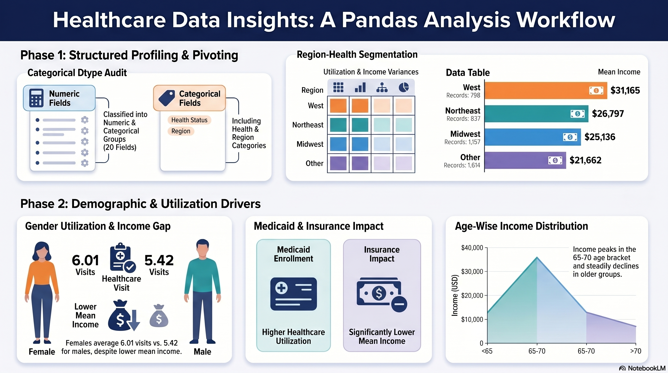
Requirement: Import Pandas, load `NSMES1988updated.csv`, and create the working dataframe.

Capstone 3 begins from the Capstone 2 handoff artifact and uses a path fallback so the notebook can resolve the updated dataset from the prior capstone output.

Results Capture

Main input: `Capstone 2/outputs/NSMES1988updated.csv`.
Working dataframe shape: `(4406, 20)` with the `age_years` and `income_dollars` columns already present from Capstone 2.
Analysis starts from the updated handoff file.

import pandas as pd

DEFAULT_DATASET = "NSMES1988updated.csv"

try:
    dataset_path = resolve_dataset_path(DEFAULT_DATASET)
except FileNotFoundError:
    fallback = first_existing_path([
        BASE_DIR.parent / "Capstone 2" / "outputs" / "NSMES1988updated.csv",
        CWD / "Capstone 2" / "outputs" / "NSMES1988updated.csv",
        CWD / "Incremental_Capstone" / "Capstone 2" / "outputs" / "NSMES1988updated.csv",
    ])
    if fallback is None:
        raise
    dataset_path = fallback

df = pd.read_csv(dataset_path)
print("Loaded:", dataset_path)
print("Shape:", df.shape)
display(df.head())

Audit Data Types And Identify Categorical Fields

Notebook section: C3-T4

Requirement: Identify different data types and identify categorical types in the data.

The notebook produces a full dtype audit and then confirms which fields must be treated as categories rather than continuous numeric measures.

Results Capture

A 20-column dtype audit table is created with a `data_type_group` classification.
`health` categories: `average`, `excellent`, `poor`.
`region` categories: `midwest`, `northeast`, `other`, `west`.

categorical_cols = {"health", "adl", "region", "gender", "married", "employed", "insurance", "medicaid"}
dtype_audit = pd.DataFrame({
    "column": df.columns,
    "dtype": [str(df[c].dtype) for c in df.columns],
    "data_type_group": ["categorical/flag" if c in categorical_cols else "numeric" for c in df.columns]
})
display(dtype_audit)

for col in ["health", "region"]:
    print(sorted(df[col].dropna().unique().tolist()))

Perform Detailed Pivoting For Health And Region

Notebook section: C3-T5

Requirement: Perform detailed pivoting and include Health and Region categorical analysis.

The core segmented analysis uses `region × health` pivot tables to measure record counts, average visits, and average income across the required categorical dimensions.

Results Capture

Pivot count size: `(4, 3)` covering all 4,406 records.
Three pivot outputs are generated: counts, mean visits, and mean `income_dollars`.
The pivots make the region-health utilization and income differences explicit in one place.

pivot_count = pd.pivot_table(df, index="region", columns="health", values="visits", aggfunc="count", fill_value=0)
pivot_mean_visits = pd.pivot_table(df, index="region", columns="health", values="visits", aggfunc="mean", fill_value=0)
pivot_mean_income = pd.pivot_table(df, index="region", columns="health", values="income_dollars", aggfunc="mean", fill_value=0)

display(pivot_count)
display(pivot_mean_visits.round(3))
display(pivot_mean_income.round(2))

Analyze Required Criteria Tables

Notebook section: C3-T6

Requirement: Analyze visits, gender, marital status, school, income, employment status, insurance, and medical aid.

Capstone 3 groups utilization and income metrics by each requested demographic and coverage criterion so the requested comparison tables stay directly aligned to the PDF.

Results Capture

Grouped criteria tables are produced for `gender`, `married`, `school`, `employed`, `insurance`, and `medicaid`.
Female mean visits exceed male mean visits in the notebook summary, while male mean income is higher.
Medicaid enrollment aligns with higher mean visits and lower mean income in the staged notebook output.

criteria_cols = ["gender", "married", "school", "employed", "insurance", "medicaid"]
metric_cols = [c for c in ["visits", "nvisits", "ovisits", "novisits", "emergency", "hospital"] if c in df.columns]

for c in criteria_cols:
    table = df.groupby(c)[metric_cols + ["income_dollars"]].mean(numeric_only=True).round(3)
    display(table)

Build The Required Distribution Tables And Findings

Notebook section: C3-T7 and conclusions

Requirement: Create age and gender, health by gender, income by gender, regional income, and age-wise income distributions and report findings.

The notebook closes the capstone by building all required distribution tables and then documenting the cross-group patterns that matter for the report.

Results Capture

Required distribution table sizes reported in the notebook: Age+Gender `(5x2)`, Health by Gender `(3x2)`, Income by Gender `(2x3)`, Regional Income `(4x3)`, Age-wise Income `(5x3)`.
The notebook notes that `west` shows the highest regional mean income and `other` the lowest.
The conclusion section confirms the PDF-required segmented analysis was completed and written up in the notebook markdown.

df3 = df.copy()
df3["age_group"] = pd.cut(df3["age_years"].astype(float), bins=[65, 70, 75, 80, 85, 110], include_lowest=True)

display(pd.crosstab(df3["age_group"], df3["gender"]))
display(pd.crosstab(df3["health"], df3["gender"]))
display(pd.pivot_table(df3, index="gender", values="income_dollars", aggfunc=["count", "mean", "median"]).round(2))
display(pd.pivot_table(df3, index="region", values="income_dollars", aggfunc=["count", "mean", "median"]).round(2))
display(pd.pivot_table(df3, index="age_group", values="income_dollars", aggfunc=["count", "mean", "median"]).round(2))

Data And Artifact Links

The links below open the Capstone 3 project files.

Artifact

Original Project PDF

View the copied Capstone 3 directions PDF used as the source requirement document.

View Download

Artifact

Notebook Evidence

Open the Capstone 3 notebook in the browser-friendly artifact viewer.

View Download

Artifact

Requirements Checklist

Open the Capstone 3 requirements file created from the copied PDF task list.

View Download

Artifact

Reference Source CSV

Open the original `NSMES1988.csv` source copy kept with Capstone 3.

View Download

Artifact

Capstone 2 Updated Input CSV

Open the `NSMES1988updated.csv` handoff dataset used as the Capstone 3 notebook input.

View Download

Artifact

Project Infographic

Open the user-supplied Capstone 3 infographic asset.

View Download

Colab Notebook

This section provides the notebook preview, launch link, and project file links.

The notebook preview is the primary execution record for this capstone.

Embedded Notebook Preview

Cell 1 Markdown

Capstone 3 — Session 3: Data Analysis with Pandas

Run timestamp: 2026-02-19 01:49:22

Goal

Perform structured exploratory analysis on the Capstone 2 processed dataset using categorical profiling, pivot analysis, and distribution tables.
Produce interpretable tables for health, region, demographic, and income patterns to support downstream business insights.

Inputs

NSMES1988updated.csv (primary source from Capstone 2/outputs/)

Outputs

All exports go to ./outputs/ (and plots to ./outputs/plots/ when applicable)

Libraries (documented)

pandas: needed for pivots, crosstabs, grouping, and distribution tables; enabled all required session analyses.

Key dataset note

age is encoded as Age in years (divided by 10) (e.g., 6.9 = 69 years).

Cell 2 Markdown

C?-T0 — Runtime setup (paths + output folders)

I used this setup block first to configure reproducible paths and output folders.

Cell 3 Code · python

from pathlib import Path
from datetime import datetime
from urllib.parse import quote
from urllib.request import urlretrieve
import os
import sys

try:
    from IPython.display import display
except Exception:
    def display(value):
        print(value)

# --- Project metadata ---
CAPSTONE = 3
SESSION_TITLE = 'Session 3: Data Analysis with Pandas'
IS_COLAB = 'google.colab' in sys.modules
RAW_BASE = os.environ.get('FRANCISBURNET_RAW_BASE', 'https://raw.githubusercontent.com/FrancisBurnet/francisburnet/main')

print(f"Capstone: {CAPSTONE} | Session: {SESSION_TITLE}")
print("Run timestamp:", datetime.now().strftime("%Y-%m-%d %H:%M:%S"))
print("Runtime:", "Google Colab" if IS_COLAB else "Local / notebook runtime")

CWD = Path.cwd()
if IS_COLAB:
    BASE_DIR = Path('/content/francisburnet_capstone_3')
elif (CWD / f"Capstone {CAPSTONE}").exists():
    BASE_DIR = CWD / f"Capstone {CAPSTONE}"
elif CWD.name == f"Capstone {CAPSTONE}":
    BASE_DIR = CWD
elif (CWD / 'Incremental_Capstone' / f"Capstone {CAPSTONE}").exists():
    BASE_DIR = CWD / 'Incremental_Capstone' / f"Capstone {CAPSTONE}"
elif (CWD / 'Incremental Capstones' / 'Applied Data Science with Python' / f"Capstone {CAPSTONE}").exists():
    BASE_DIR = CWD / 'Incremental Capstones' / 'Applied Data Science with Python' / f"Capstone {CAPSTONE}"
else:
    BASE_DIR = CWD

INPUT_DIR = BASE_DIR / 'inputs'
OUTPUT_DIR = BASE_DIR / 'outputs'
PLOTS_DIR = OUTPUT_DIR / 'plots'
INPUT_DIR.mkdir(parents=True, exist_ok=True)
OUTPUT_DIR.mkdir(parents=True, exist_ok=True)
PLOTS_DIR.mkdir(parents=True, exist_ok=True)

def first_existing_path(candidates):
    for candidate in candidates:
        candidate = Path(candidate).expanduser()
        if candidate.exists():
            return candidate
    return None

def github_raw_url(relative_path: str) -> str:
    normalized = relative_path.replace('\\', '/')
    return RAW_BASE.rstrip('/') + '/' + quote(normalized, safe='/')

def stage_colab_asset(relative_path: str, destination_name=None) -> Path:
    destination = INPUT_DIR / (destination_name or Path(relative_path).name)
    if not destination.exists():
        asset_url = github_raw_url(relative_path)
        urlretrieve(asset_url, destination)
        print('Downloaded:', destination.name, 'from', asset_url)
    return destination

LOCAL_SEARCH_ROOTS = [
    INPUT_DIR,
    BASE_DIR,
    CWD,
    CWD / f"Capstone {CAPSTONE}",
    CWD / 'Incremental_Capstone' / f"Capstone {CAPSTONE}",
    CWD / 'Incremental Capstones' / 'Applied Data Science with Python' / f"Capstone {CAPSTONE}",
    CWD.parent / 'Incremental_Capstone' / f"Capstone {CAPSTONE}",
    CWD.parent / 'Incremental Capstones' / 'Applied Data Science with Python' / f"Capstone {CAPSTONE}",
]

def resolve_dataset_path(default_filename: str) -> Path:
    candidates = [Path(root) / default_filename for root in LOCAL_SEARCH_ROOTS]
    path = first_existing_path(candidates)
    if path is None:
        searched_paths = [str(candidate) for candidate in candidates]
        raise FileNotFoundError(f"Dataset not found: {default_filename}. Searched: {searched_paths}")
    return path

if IS_COLAB:
    staged_assets = [
        'Incremental Capstones/Applied Data Science with Python/Capstone 3/Capstone_Session_3.pdf',
        'Incremental Capstones/Applied Data Science with Python/Capstone 3/NSMES1988.csv',
        'Incremental Capstones/Applied Data Science with Python/Capstone 3/capstone_3.ipynb',
    ]
    for relative_path in staged_assets:
        stage_colab_asset(relative_path)

print('Base directory:', BASE_DIR)
print('Input directory:', INPUT_DIR)
print('Output directory:', OUTPUT_DIR)
print('Plots directory:', PLOTS_DIR)

Output

Capstone: 3 | Session: Session 3: Data Analysis with Pandas
Run timestamp: 2026-05-12 03:57:44
Runtime: Local / notebook runtime
Base directory: x:\SIMPLILEARN\FrancisBurnetCom\Incremental Capstones\Applied Data Science with Python\Capstone 3
Input directory: x:\SIMPLILEARN\FrancisBurnetCom\Incremental Capstones\Applied Data Science with Python\Capstone 3\inputs
Output directory: x:\SIMPLILEARN\FrancisBurnetCom\Incremental Capstones\Applied Data Science with Python\Capstone 3\outputs
Plots directory: x:\SIMPLILEARN\FrancisBurnetCom\Incremental Capstones\Applied Data Science with Python\Capstone 3\outputs\plots

Cell 4 Markdown

C?-T1 — Imports I used

I documented each import with why I used it and what it enabled in this analysis.

Cell 5 Code · python

import pandas as pd  # DataFrames + pivot/crosstab/groupby analysis for categorical and distribution tables

Cell 6 Markdown

C?-T2 — Load dataset

I loaded the required Capstone 3 dataset with the configured default and fallback path.

Cell 7 Code · python

DEFAULT_DATASET = 'NSMES1988updated.csv'

fallback_candidates = [
    BASE_DIR.parent / 'Capstone 2' / 'outputs' / DEFAULT_DATASET,
    CWD / 'Capstone 2' / 'outputs' / DEFAULT_DATASET,
    CWD / 'Incremental_Capstone' / 'Capstone 2' / 'outputs' / DEFAULT_DATASET,
    CWD / 'Incremental Capstones' / 'Applied Data Science with Python' / 'Capstone 2' / 'outputs' / DEFAULT_DATASET,
    CWD.parent / 'Incremental_Capstone' / 'Capstone 2' / 'outputs' / DEFAULT_DATASET,
    CWD.parent / 'Incremental Capstones' / 'Applied Data Science with Python' / 'Capstone 2' / 'outputs' / DEFAULT_DATASET,
]

try:
    dataset_path = resolve_dataset_path(DEFAULT_DATASET)
except FileNotFoundError:
    fallback = first_existing_path(fallback_candidates)
    if fallback is None and IS_COLAB:
        fallback = stage_colab_asset(
            'Incremental Capstones/Applied Data Science with Python/Capstone 2/outputs/NSMES1988updated.csv'
        )
    if fallback is None:
        searched_paths = [str(candidate) for candidate in fallback_candidates]
        raise FileNotFoundError(f"Dataset not found: {DEFAULT_DATASET}. Searched: {searched_paths}")
    dataset_path = fallback
    print('Default dataset not found; using fallback:', dataset_path)

df = pd.read_csv(dataset_path)

print('Loaded:', dataset_path)
print('Shape:', df.shape)
display(df.head())

Output

Local default not found; using fallback: c:\DEV_Projects\SIMPLILEARN\CAPSTONE_Applied_Data_Science_with _Python\Incremental_Capstone\Capstone 2\outputs\NSMES1988updated.csv
Loaded: c:\DEV_Projects\SIMPLILEARN\CAPSTONE_Applied_Data_Science_with _Python\Incremental_Capstone\Capstone 2\outputs\NSMES1988updated.csv
Shape: (4406, 20)

   visits  nvisits  ovisits  novisits  emergency  hospital   health  chronic  \
0       5        0        0         0          0         1  average        2   
1       1        0        2         0          2         0  average        2   
2      13        0        0         0          3         3     poor        4   
3      16        0        5         0          1         1     poor        2   
4       3        0        0         0          0         0  average        2   

       adl region  age  gender married  school  income employed insurance  \
0   normal  other  6.9    male     yes       6  2.8810      yes       yes   
1   normal  other  7.4  female     yes      10  2.7478       no       yes   
2  limited  other  6.6  female      no      10  0.6532       no        no   
3  limited  other  7.6    male     yes       3  0.6588       no       yes   
4  limited  other  7.9  female     yes       6  0.6588       no       yes   

  medicaid  age_years  income_dollars  
0       no         69           28810  
1       no         74           27478  
2      yes         66            6532  
3       no         76            6588  
4       no         79            6588

Cell 8 Markdown

C?-T3 — Validation checks

I confirmed expected columns exist
I confirmed key dtypes
I checked missing values

Results Capture:

What I did: I validated expected Capstone 3 schema from Capstone 2 output, checked dtypes, and computed missing values.
What I found: dataframe loaded as (4406, 20) with all expected columns including age_years and income_dollars; total missing values = 0.
Caveats: label columns (health, region, gender, married, employed, insurance, medicaid) are categorical and should not be interpreted as continuous numeric values.

Cell 9 Code · python

expected_cols = [
    "visits", "nvisits", "ovisits", "novisits", "emergency", "hospital",
    "health", "chronic", "adl", "region", "age", "gender",
    "married", "school", "income", "employed", "insurance", "medicaid",
    "age_years", "income_dollars"
]

missing_cols = [c for c in expected_cols if c not in df.columns]
print("Missing expected columns:", missing_cols)

print("\nDtypes:")
display(df.dtypes)

print("\nMissing values (count):")
na_counts = df.isna().sum().sort_values(ascending=False)
display(na_counts[na_counts > 0] if (na_counts > 0).any() else na_counts.head())

Output

Missing expected columns: []

Dtypes:

visits              int64
nvisits             int64
ovisits             int64
novisits            int64
emergency           int64
hospital            int64
health                str
chronic             int64
adl                   str
region                str
age               float64
gender                str
married               str
school              int64
income            float64
employed              str
insurance             str
medicaid              str
age_years           int64
income_dollars      int64
dtype: object

Missing values (count):

visits       0
nvisits      0
ovisits      0
novisits     0
emergency    0
dtype: int64

Cell 10 Markdown

C3-T4 — Identify categorical types + key categories

PDF requirement: Identify different types of data and identify categorical types.

What I completed

I audited dtypes, grouped variables by type, and listed unique category values for health and region.

Results Capture

Built a type-audit table (column, dtype, data_type_group) for all 20 columns.
health categories: ['average', 'excellent', 'poor'].
region categories: ['midwest', 'northeast', 'other', 'west'].

Code evidence

The next cell shows the dtype audit and category-value extraction I executed.

Cell 11 Code · python

categorical_cols = {"health", "adl", "region", "gender", "married", "employed", "insurance", "medicaid"}
dtype_audit = pd.DataFrame({
    "column": df.columns,
    "dtype": [str(df[c].dtype) for c in df.columns],
    "data_type_group": ["categorical/flag" if c in categorical_cols else "numeric" for c in df.columns]
})
display(dtype_audit)

for col in ["health", "region"]:
    if col in df.columns:
        print(f"\nUnique values for {col}:")
        print(sorted(df[col].dropna().unique().tolist()))

Output

            column    dtype   data_type_group
0           visits    int64           numeric
1          nvisits    int64           numeric
2          ovisits    int64           numeric
3         novisits    int64           numeric
4        emergency    int64           numeric
5         hospital    int64           numeric
6           health      str  categorical/flag
7          chronic    int64           numeric
8              adl      str  categorical/flag
9           region      str  categorical/flag
10             age  float64           numeric
11          gender      str  categorical/flag
12         married      str  categorical/flag
13          school    int64           numeric
14          income  float64           numeric
15        employed      str  categorical/flag
16       insurance      str  categorical/flag
17        medicaid      str  categorical/flag
18       age_years    int64           numeric
19  income_dollars    int64           numeric

Unique values for health:
['average', 'excellent', 'poor']

Unique values for region:
['midwest', 'northeast', 'other', 'west']

Cell 12 Markdown

C3-T5 — Pivoting including Health and Region

PDF requirement: Perform detailed pivoting and include categorical data analysis for Health and Region.

What I completed

I generated pivot tables for counts, mean visits, and mean income by region and health.

Results Capture

Generated 3 detailed pivots by region × health: count matrix, mean visits, and mean income (dollars).
Pivot count size = (4, 3) and total records represented = 4406.
Interpretation highlights:
All four regions contain observations across all three health categories.
Mean utilization varies by region-health combinations, supporting segmented analysis.
Mean income differences by region-health indicate socio-economic heterogeneity across segments.

Code evidence

The next cell contains the exact pivot computations and displayed outputs.

Cell 13 Code · python

# Region-health pivots (counts + average visits + average income)
if set(["region", "health"]).issubset(df.columns):
    pivot_count = pd.pivot_table(df, index="region", columns="health", values="visits", aggfunc="count", fill_value=0)
    pivot_mean_visits = pd.pivot_table(df, index="region", columns="health", values="visits", aggfunc="mean", fill_value=0)
    pivot_mean_income = pd.pivot_table(df, index="region", columns="health", values="income_dollars", aggfunc="mean", fill_value=0)
    print("Pivot 1: Count by region x health")
    display(pivot_count)
    print("Pivot 2: Mean visits by region x health")
    display(pivot_mean_visits.round(3))
    print("Pivot 3: Mean income_dollars by region x health")
    display(pivot_mean_income.round(2))

Output

Pivot 1: Count by region x health

health     average  excellent  poor
region                             
midwest        957         90   110
northeast      694         57    86
other         1237        105   272
west           621         91    86

Pivot 2: Mean visits by region x health

health     average  excellent    poor
region                               
midwest      5.282      3.444   8.118
northeast    5.695      4.018  10.674
other        5.088      3.143   8.746
west         6.499      3.374   8.593

Pivot 3: Mean income_dollars by region x health

health      average  excellent      poor
region                                  
midwest    24984.23   31053.89  21618.12
northeast  27015.35   33400.12  20659.30
other      22010.96   30024.58  16851.79
west       31663.77   37255.87  21118.85

Cell 14 Markdown

C3-T6 — Criteria-based analysis (visits, gender, marital, school, income, employed, insurance, medicaid)

PDF requirement: Analyze the data based on multiple criteria including visits type, gender, marital status, school, income, employed, insurance, medical aid.

What I completed

I produced grouped mean tables for each requested criterion across utilization and income metrics.

Results Capture

Produced one compact mean table per criterion (gender, married, school, employed, insurance, medicaid) for visit metrics and income_dollars.
Key findings:
gender: mean visits female=6.014 vs male=5.420; mean income female=22,493.476, male=29,377.156.
insurance: insured group has higher mean visits (6.023) than uninsured (4.913).
medicaid: enrollment corresponds to higher mean visits (6.714) but lower mean income (11,365.388) vs non-enrolled.

Code evidence

The next cell shows all criterion-based grouped tables I generated.

Cell 15 Code · python

criteria_cols = ["gender", "married", "school", "employed", "insurance", "medicaid"]
metric_cols = [c for c in ["visits", "nvisits", "ovisits", "novisits", "emergency", "hospital"] if c in df.columns]

print("Metric columns guess:", metric_cols)

for c in criteria_cols:
    if c in df.columns and metric_cols:
        print(f"\nCriteria table: {c}")
        table = df.groupby(c)[metric_cols + ["income_dollars"]].mean(numeric_only=True).round(3)
        display(table)

Output

Metric columns guess: ['visits', 'nvisits', 'ovisits', 'novisits', 'emergency', 'hospital']

Criteria table: gender

        visits  nvisits  ovisits  novisits  emergency  hospital  \
gender                                                            
female   6.014    1.732    0.683     0.513      0.269     0.286   
male     5.420    1.449    0.851     0.570      0.255     0.311   

        income_dollars  
gender                  
female       22493.476  
male         29377.156

Criteria table: married

         visits  nvisits  ovisits  novisits  emergency  hospital  \
married                                                            
no        5.932    1.549    0.650     0.507      0.302     0.311   
yes       5.644    1.675    0.835     0.560      0.232     0.283   

         income_dollars  
married                  
no            17194.294  
yes           31985.391

Criteria table: school

        visits  nvisits  ovisits  novisits  emergency  hospital  \
school                                                            
0        4.214    0.806    1.748     1.709      0.282     0.340   
1        5.538    0.154    0.385     0.077      0.231     0.462   
2        5.079    0.184    0.421     0.263      0.184     0.342   
3        6.239    0.535    1.014     0.296      0.662     0.423   
4        4.750    0.910    0.520     0.180      0.320     0.260   
5        5.854    0.417    0.718     0.058      0.350     0.359   
6        5.358    1.116    0.428     1.006      0.353     0.341   
7        5.448    0.982    0.529     0.457      0.285     0.285   
8        5.582    1.431    0.785     0.507      0.281     0.307   
9        4.795    1.043    0.765     0.436      0.333     0.380   
10       5.696    1.913    0.817     0.554      0.315     0.284   
11       5.789    1.599    0.938     0.339      0.264     0.233   
12       5.887    1.932    0.776     0.574      0.222     0.304   
13       6.378    1.866    0.488     0.372      0.331     0.291   
14       6.126    1.828    0.504     0.483      0.206     0.227   
15       7.081    1.663    0.535     0.605      0.105     0.186   
16       6.092    2.616    0.900     0.592      0.184     0.248   
17       6.478    3.065    0.761     0.391      0.152     0.196   
18       7.887    1.915    0.679     0.500      0.151     0.274   

        income_dollars  
school                  
0            21664.155  
1            12929.154  
2            13085.395  
3            14183.507  
4            13851.000  
5            14735.214  
6            17893.104  
7            16157.104  
8            20111.042  
9            18457.111  
10           19863.163  
11           21885.476  
12           27290.700  
13           29762.744  
14           32537.803  
15           34549.686  
16           43962.132  
17           51312.761  
18           54112.377

Criteria table: employed

          visits  nvisits  ovisits  novisits  emergency  hospital  \
employed                                                            
no         5.807    1.640    0.786     0.549      0.269     0.304   
yes        5.495    1.426    0.444     0.424      0.220     0.226   

          income_dollars  
employed                  
no             23600.560  
yes            39779.402

Criteria table: insurance

           visits  nvisits  ovisits  novisits  emergency  hospital  \
insurance                                                            
no          4.913    0.934    1.056     0.436      0.333     0.311   
yes         6.023    1.815    0.663     0.565      0.243     0.292   

           income_dollars  
insurance                  
no              16629.839  
yes             27759.441

Criteria table: medicaid

          visits  nvisits  ovisits  novisits  emergency  hospital  \
medicaid                                                            
no         5.680    1.654    0.725     0.534      0.246     0.284   
yes        6.714    1.259    1.007     0.555      0.443     0.415   

          income_dollars  
medicaid                  
no             26667.471  
yes            11365.388

Cell 16 Markdown

C3-T7 — Create required distribution tables

PDF requirement: Create distribution tables: Age+Gender; Health by Gender; Income by Gender; Regional Income; Age-wise Income.

What I completed

I built all required distribution tables using age groups, crosstabs, and grouped income summaries.

Results Capture

Built all required distribution tables:
Age + Gender (5x2), Health by Gender (3x2), Income by Gender (2x3), Regional Income (4x3), Age-wise Income (5x3).
Notable patterns:
Regional mean income is highest in west and lowest in other.
Male mean income exceeds female mean income, while female mean visits are higher.
Older age groups remain strongly represented across both genders.

Code evidence

The next cell contains the exact table-generation logic for all required distributions.

Cell 17 Code · python

df3 = df.copy()

age_col = "age_years" if "age_years" in df3.columns else "age"
income_col = "income_dollars" if "income_dollars" in df3.columns else "income"

if age_col in df3.columns:
    df3["age_group"] = pd.cut(df3[age_col].astype(float), bins=[65, 70, 75, 80, 85, 110], include_lowest=True)

if income_col in df3.columns:
    quantiles = df3[income_col].quantile([0, .2, .4, .6, .8, 1.0]).values
    edges = [quantiles[0]]
    for value in quantiles[1:]:
        edges.append(value if value > edges[-1] else edges[-1] + 1)
    df3["income_band"] = pd.cut(df3[income_col].astype(float), bins=edges, include_lowest=True)

if set(["age_group", "gender"]).issubset(df3.columns):
    print("Distribution 1: Age + Gender")
    display(pd.crosstab(df3["age_group"], df3["gender"]))

if set(["health", "gender"]).issubset(df3.columns):
    print("Distribution 2: Health by Gender")
    display(pd.crosstab(df3["health"], df3["gender"]))

if set(["income_dollars", "gender"]).issubset(df3.columns):
    print("Distribution 3: Income by Gender")
    display(pd.pivot_table(df3, index="gender", values="income_dollars", aggfunc=["count", "mean", "median"]).round(2))

if set(["income_dollars", "region"]).issubset(df3.columns):
    print("Distribution 4: Regional Income")
    display(pd.pivot_table(df3, index="region", values="income_dollars", aggfunc=["count", "mean", "median"]).round(2))

if set(["age_group", "income_dollars"]).issubset(df3.columns):
    print("Distribution 5: Age-wise Income")
    display(pd.pivot_table(df3, index="age_group", values="income_dollars", aggfunc=["count", "mean", "median"]).round(2))

Output

Distribution 1: Age + Gender

gender          female  male
age_group                   
(64.999, 70.0]     897   671
(70.0, 75.0]       736   530
(75.0, 80.0]       525   321
(80.0, 85.0]       303   176
(85.0, 110.0]      167    80

Distribution 2: Health by Gender

gender     female  male
health                 
average      2093  1416
excellent     193   150
poor          342   212

Distribution 3: Income by Gender

                count           mean         median
       income_dollars income_dollars income_dollars
gender                                             
female           2628       22493.48        14160.0
male             1778       29377.16        20574.0

Distribution 4: Regional Income

                   count           mean         median
          income_dollars income_dollars income_dollars
region                                                
midwest             1157       25136.34        17875.0
northeast            837       26797.09        17413.0
other               1614       21662.84        14220.0
west                 798       31165.05        20656.0

Distribution 5: Age-wise Income

                        count           mean         median
               income_dollars income_dollars income_dollars
age_group                                                  
(64.999, 70.0]           1568       27488.76        19872.0
(70.0, 75.0]             1266       26194.35        16986.0
(75.0, 80.0]              846       22997.60        15135.0
(80.0, 85.0]              479       20269.47        12886.0
(85.0, 110.0]             247       23951.36        13940.0

Cell 18 Markdown

Final section — Conclusions (required)

I used Capstone 2/outputs/NSMES1988updated.csv as the input for this analysis.
I completed categorical profiling and pivoting for health and region with clear segmentation outputs.
I documented meaningful criteria-based differences across gender, insurance, medicaid, marital status, employment, and schooling groups.
I generated and interpreted all required distribution tables.
I updated WORK_SUMMARY.md with evidence and marked all Capstone 3 tasks complete.

Cell 19 Code · python

print("Capstone 3 completed: C3-T4 to C3-T7")
print("Input used: Capstone 2/outputs/NSMES1988updated.csv")

Output

Capstone 3 completed: C3-T4 to C3-T7
Input used: Capstone 2/outputs/NSMES1988updated.csv

Project Notes

Input dataset from Capstone 2.
Dtype audit and categorical review.
Pivot, grouped analysis, and distribution tables.
Code screenshots and notebook evidence.

Project File Links

Capstone 2 Updated Input CSV: Open Capstone 2 Updated Input CSV
Primary handoff dataset loaded by the Capstone 3 notebook.
Notebook File: Open Notebook File
Staged Capstone 3 notebook used as the main evidence source for the page walkthrough.
Reference Source CSV: Open Reference Source CSV
Original NSMES source copy retained in the Capstone 3 folder for lineage reference.
Notebook Source: Open Notebook Source
Public notebook source path used when a Colab launch URL is configured.

Screenshot Evidence

Code Screenshot

Dtype Audit Code Screenshot

Captured code evidence for the dtype audit and categorical-field identification section.

View Download

Code Screenshot

Pivot Analysis Code Screenshot

Captured code evidence for the region-health pivot tables.

View Download

Code Screenshot

Distribution Tables Code Screenshot

Captured code evidence for the required distribution-table section.

View Download

Outputs And Results

Key Outputs

The notebook produces pivot tables and grouped distribution tables directly in the notebook outputs rather than exporting new CSV handoff files.
The code screenshots preserve the pivot, grouped-criteria, and distribution-table logic.
The requirements file documents the assignment task list.

Key Findings

Region-health pivoting shows measurable variation in both visits and income across segments.
The grouped criteria tables surface clear visit and income differences across insurance and medicaid status.
The required distribution tables keep the Week 3 and Week 4 reporting aligned to age, gender, region, and income patterns without inventing extra requirements.